Data Conditioning

Supported by FFT Spectral Analysis, Time-Stamp, Order-Tracking, Sine Reduction & Basic Signal-Conditioning support data conditioning features. Data Conditioning supports functions to control and process data using a logic gate structure.

Follow the guided steps below to understand and use the data conditioning functionality in Post Analyzer

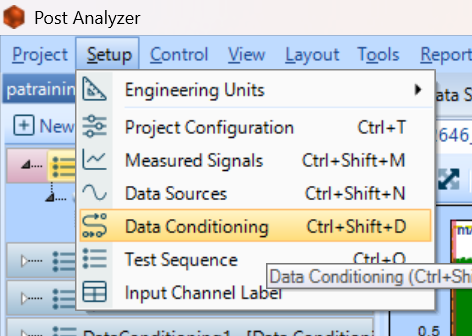
Data conditioning tabs can be opened through the Setup → Data Conditioning dropdown, or the user can press Ctr+Shift+D.

Data Conditioning has several tabs each with different module types.

Math modules include basic arithmetic operations such as Add, Subtract, Multiply, Square etc., and a few more complex operations.

Offset Scale provides a scalar multiplication and additive offset to input channel. Functions as a gain+ bias operator ThreeRectangular supports a three-element strain gauge. Calculating principal strains, stresses, angle of orientation, and max shear. Rosette supports 3-gage rosette for both 3 element and delta types. Outputs equivalent strain in x, y, and shear planes, principal plane angle, principal stress & strains, and maximum shear strain. Sound Analysis calculates sound pressure, sound intensity and vibration velocity.

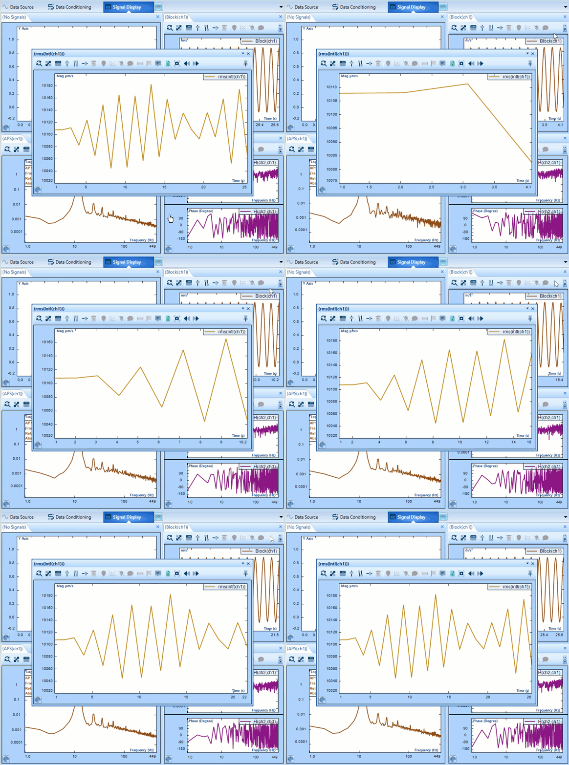
Statistics supports a variety of functions used in data interpretation. Including several common functions i.e. Min, Max, Mean. It also supports more specialized operations: Peak to Peak operator saves the greatest displacement between signal minimum and maximum of oscillation during time block. RMS calculates the effective signal strength over a period.

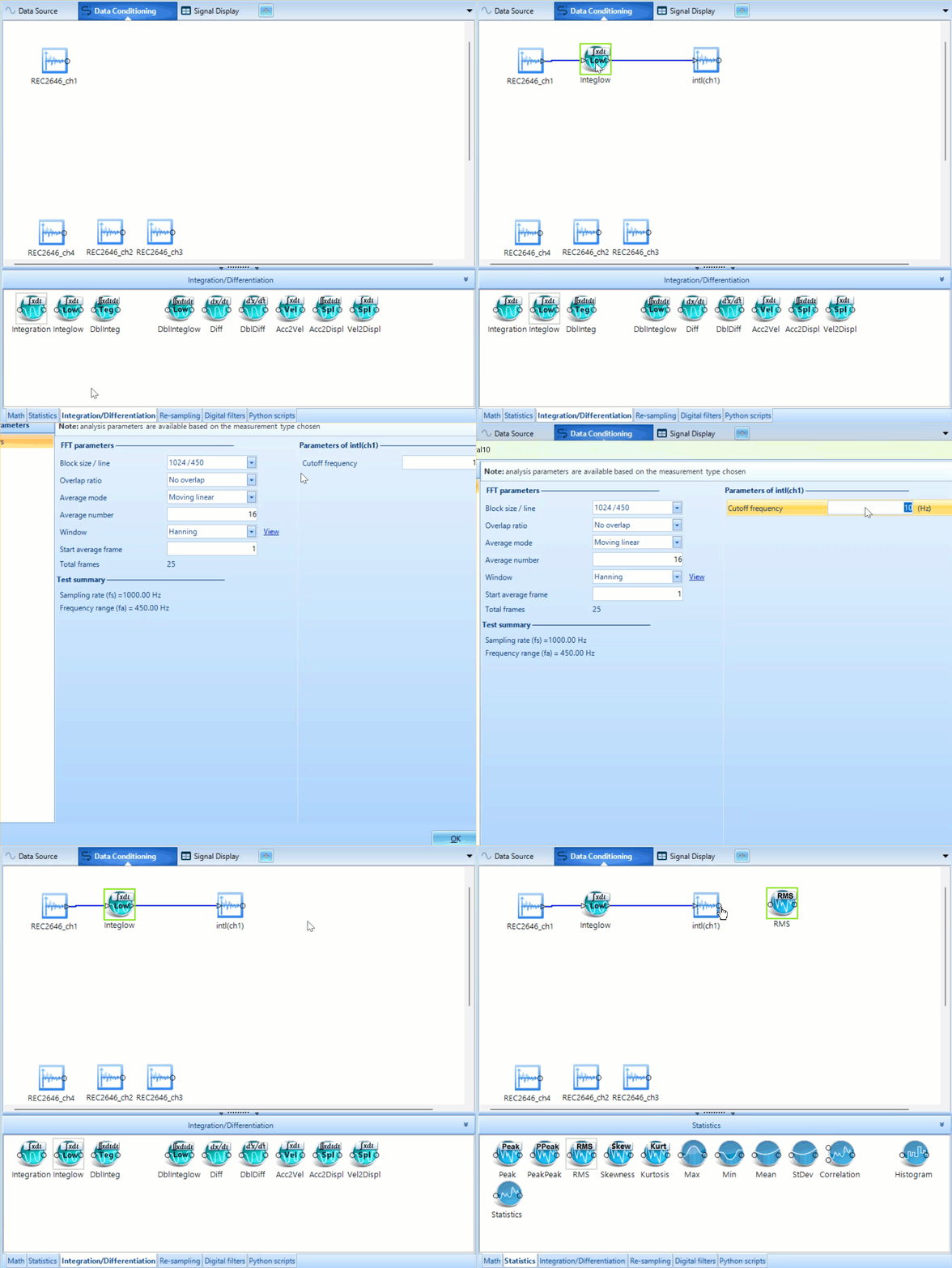
Integration/Differentiation modules behave as anticipated with a couple extra features. The modules which include the term low, such as Integlow conduct the same operation as the parent feature, Integral, but include an additional low-pass filter which can be customized by right clicking on the modules and left clicking Edit Analysis Parameter. Dblinteg works as shown in the equation, it integrates the time signal twice. The same naming standard is used for the Differentiation modules.

DecimFilter the decimator filter reduces the amount of time domain point to make computing more efficient. The data is put through a low pass anti-alias filter and then every nth point is kept. Resampling filter updates the sample to be L/M. The input time stream data is up sampled by L, there are L-1 data points filled in with zeros between time stream data input points. Next, Low pass anti-aliasing filter is applied. Finally, the data is downsampled by M. Every Mth point is kept.

Finite Impulse Response filters: Have a set time duration of response. FIR filters do not have a feedback loop and feature a constant group delay. This means that an input signal will have a uniformly delayed output and will have no distortion. FIR filters are defined by:

FIR Filter-Window is the simplest method of constructing a FIR filter. Filters are created by scaling a sinc function. It begins with a perfect passband filter and is constructed with filter coefficients to generate a desired frequency response. FIR Filter-Remez are generated from computationally intensive error reducing algorithms which reduce passband error. Infinite Impulse Response (IIR) filters are defined to last forever and decay slowly. Defined by the equation:

There is no set method of creation for IIR filters. In PA the user defines the decimation filter, filter type, filter order, analog prototype, and cutoff frequencies. Filter_RMS closely resembles the output of 1/N octave filters but with greater flexibility. Users can design any filter and examine the RMS. Functionally the same as computing the RMS after applying an RMS filter.